LLaDA: Large Language Diffusion Models
LLaDA (Large Language Diffusion with mAsking) (Nie et al. 2025) is the first full-fledged Diffusion Language Model (DLLM) that scaled the masked diffusion language model (MDLM) (Sahoo et al. 2024) formulation to 8B parameters and achieved performance comparable to Autoregressive (AR) LLMs. While MDLM provided the core of the formulation, LLaDA is a report that comprehensively shows “what happens when the formulation is reduced to an implementation,” with the concrete implementation of sampling strategies and the Supervised Fine-Tuning (SFT) for instruction-following occupying the center of the paper.
Why You Should Read LLaDA
MDLM expresses DLLM training with an extremely concise objective: a “weighted BERT training.” However, the following questions on the implementation side cannot be read off from the MDLM paper alone:
- Can we obtain scaling comparable to AR LLMs when trained at 8B scale?
- How should the inference loop after training be designed?
- Can instruction-following be SFT’d in the same way as AR?
LLaDA provides the most detailed answers currently available to these questions. This chapter focuses in particular on the inference loop and sampling strategies, and offers signposts for reading the paper.
LLaDA inherits the MDLM formulation while making the extremely straightforward choice of absorbing transition + \(x_0\)-prediction CE. Rather than novel mathematical contributions, its main contributions are scale and implementation choices.
Key Elements to Grasp
Overview of the Sampling Procedure
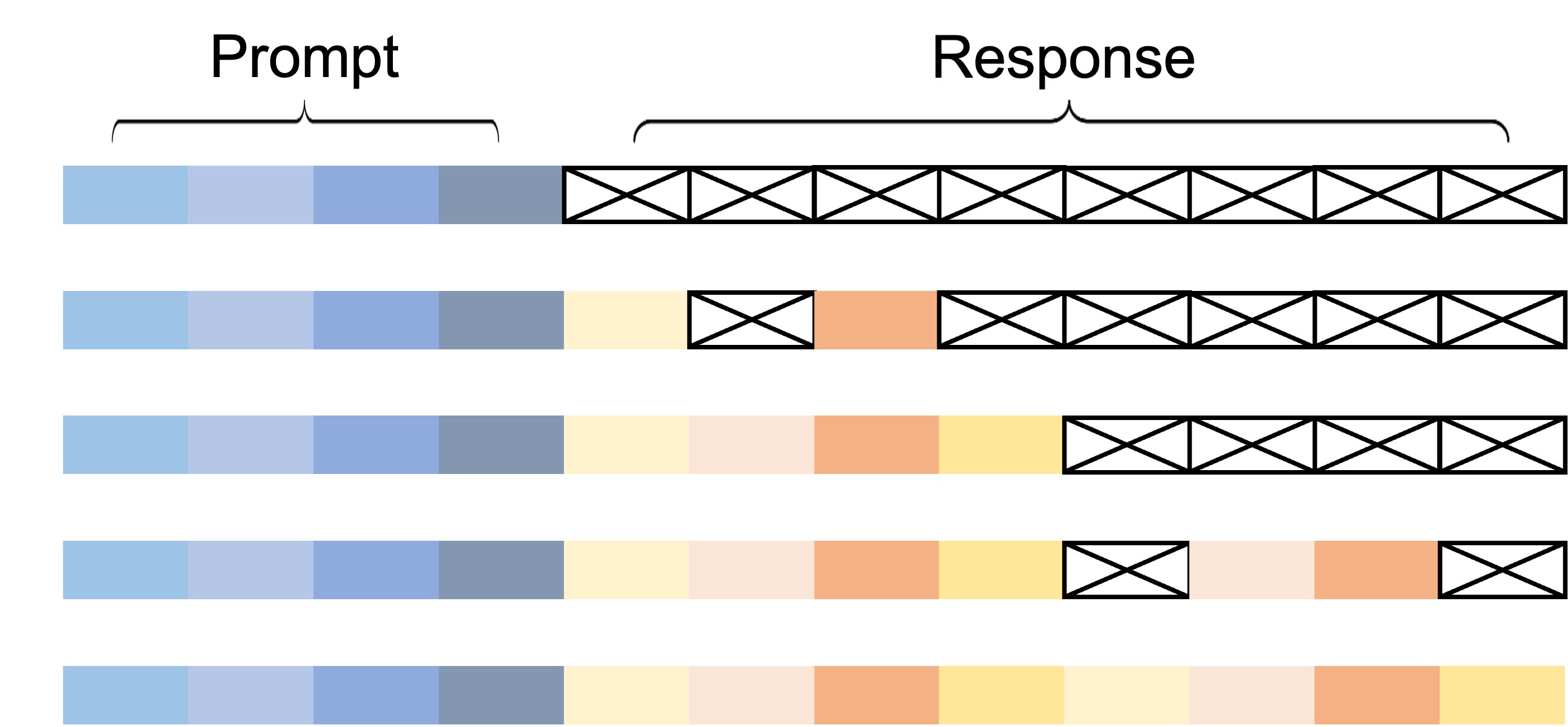
LLaDA’s inference is fundamentally different from the left-to-right loop of AR LLMs. All positions are initialized with [MASK], and at each step predictions are made for all positions, with positions of higher confidence being sequentially fixed.
One step of this loop can be written in pseudocode as follows:
# x: current token sequence (some [MASK], some already fixed)
# steps: total number of steps T
# k_t: number of positions to unmask at step t

for t in range(T, 0, -1):
    # 1. forward pass: obtain distributions over all positions
    logits = model(x)                        # [seq_len, vocab_size]
    probs = softmax(logits)

    # 2. compute confidence only for masked positions
    mask_positions = (x == MASK_ID)
    pred_tokens = argmax(probs, dim=-1)      # prediction at each position
    confidence = max(probs, dim=-1)          # confidence at each position

    # 3. unmask the top-k_t most confident masked positions
    masked_conf = confidence[mask_positions]
    topk_idx = topk(masked_conf, k_t)
    x[topk_idx] = pred_tokens[topk_idx]

    # 4. remaining masked positions stay as [MASK]
    #    (with low-confidence remasking, already-fixed positions can also be remasked)
The points are the following three:
- A forward pass is run every single step (a naive port of AR’s Key-Value (KV) cache does not work)
- The order of fixing is not left-to-right but in descending order of confidence
- The number to unmask per step \(k_t\) is determined by a schedule (linear, cosine, etc.)
Schedule of the Unmask Count \(K_t\)
How many positions to unmask at step \(t\) follows a predetermined schedule. Representative choices are as follows.
- Linear schedule: \(k_t = L/T\) constant. The same number is fixed at each step
- Cosine schedule: Sparse at the beginning and end, dense in the middle. Derived from MaskGIT and standard in image generation
- Exponential schedule: More unmasking later. A design that ensures the quality of positions fixed early
The relationship between the total number of steps \(T\) and the sequence length \(L\) can be selected continuously from \(T = L\) (1 per step) to \(T \ll L\) (many per step). The smaller \(T\) is, the faster inference is, but quality degrades because opportunities for error correction decrease.
Low-Confidence Remasking
The core of LLaDA’s implementation in practice is a strategy called low-confidence remasking. Even positions that have been unmasked once can be returned to [MASK] if they are judged to be of lower confidence than other positions in subsequent steps.
In the mathematical model, the reverse process of the absorbing transition only defines a “one-way transition from [MASK] to non-[MASK].” Theoretically, a once-unmasked position does not return. Why is remasking nevertheless performed in implementations?
The reasons for the gap between theory and implementation are as follows:
- Necessity of error correction: Positions that were fixed with low confidence at early steps become evidently incorrect as later context becomes visible. By remasking and re-incorporating information from other positions, an opportunity for correction is obtained
- Consistency with the training distribution: Since training is performed BERT-style with arbitrary mask rates \(t \in [0,1]\), passing partially-masked states through the model again at inference time remains within the training distribution
- Decoupling from the mask schedule: By separating the mathematical schedule (time \(t\)) from the implementation schedule (how many to actually unmask), the trade-off between step count and quality can be tuned on the implementation side
The absorbing diffusion formulation is only a tool for deriving the training objective, and the inference-time sampling strategy can be treated separately. The MDLM evidence lower bound (ELBO) is a “variational lower bound on the forward process” and does not prescribe the inference loop itself. It clarifies the picture to understand LLaDA as designing the inference loop independently of ELBO optimization.
Semi-Autoregressive Sampling
LLaDA further proposes a strategy called semi-autoregressive sampling. Rather than generating the whole sequence in parallel at once, it generates block by block.
- Split the sequence into blocks \(B_1, B_2, \dots, B_M\)
- Within a block, unmask in parallel as in DLLM
- Across blocks, proceed sequentially as in AR (complete \(B_1\) before moving to \(B_2\))
The intent of this design is as follows:
- Preservation of AR LLM-like flavor: Prevents the breakdown of global consistency that tends to occur in long sequences, maintaining the causal flow from left to right
- Use of KV-cache: Already-fixed blocks can be placed in the KV-cache, accelerating forward passes for subsequent blocks
- Tuning the quality/parallelism trade-off: Block size offers a continuous choice between AR-leaning (small blocks) and parallel-leaning (large blocks)
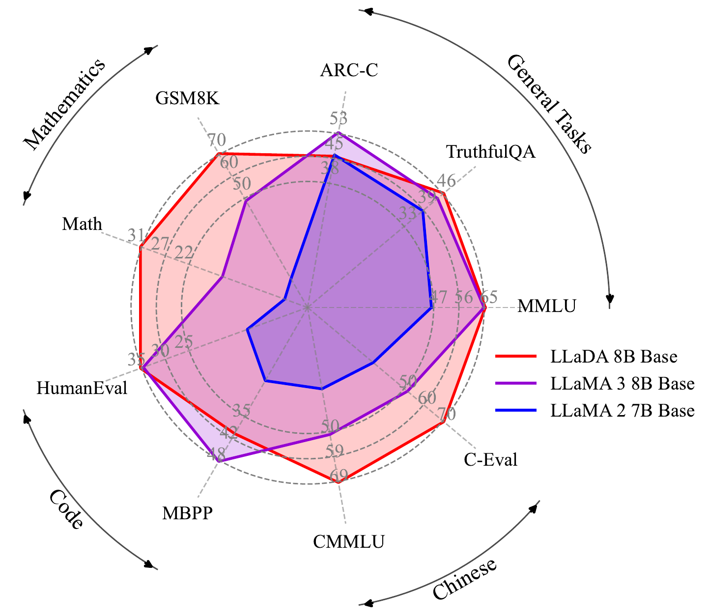
Scaling Curves
The middle of the LLaDA paper is devoted to empirically demonstrating that the 8B model scales comparably to AR LLMs. On standard benchmarks such as GSM8K, MATH, MMLU, HumanEval, and BBH, scores on par with AR LLMs of similar training compute are obtained.
| Aspect | Observation |
|---|---|
| Scaling exponent | Performance improves with an exponent nearly identical to AR LLMs |
| In-context learning | Few-shot performance also emerges on par with AR |
| Reasoning tasks (math, etc.) | Reaches the same range as AR LLMs of comparable size |
| Computational efficiency (at inference) | Depends on the number of steps \(T\). Parallelism pays off when \(T \ll L\) |
We refer to the paper for specific numbers, but the point is the establishment of the fact that “DLLMs are viable as an alternative to AR LLMs in terms of scaling laws.”
SFT for Instruction-Following
How to instruction-tune a masked DLM requires devices different from the SFT of AR LLMs. LLaDA adopts the following strategy:
- Prompt-response format: The input is given as
prompt + [MASK]*L, and only the response part is targeted for masking - Mask-rate schedule: At training time the mask rate \(t\) is sampled uniformly from \([0,1]\) (same as pretraining). The state where the entire response is
[MASK](\(t=1\)) is also included - Loss computation: The cross-entropy weight \(1/t\) is the same as in pretraining, and no SFT-specific loss is introduced
In other words, SFT is implemented as “a conditional training that is an extension of pretraining, with the prompt as a condition.” Structurally, this corresponds to AR LLM SFT “limiting the next-token prediction loss to only the response part.”
The prompt is given as always observed (not masked), and only the response part is the target of diffusion. This is the same idea as AR LLMs giving the prompt as context and computing the loss only over the response part.
Reading Priority (Paper Sections)
The paper is large in scale, so it is efficient to narrow the reading order to your purpose.
| Section | Importance | Content |
|---|---|---|
| §2 formulation | Must read | Confirm that the formulation is nearly identical to MDLM |
| §3 sampling | Most important (two or more passes) | Implementation details of the inference loop, remasking, and semi-AR |
| §4 results | Scan | Scaling results and comparison with other models |
| §5 analyses | As interested | Detailed analyses of mask-rate effects, step count effects, etc. |
§2 Formulation (Must Read)
It is sufficient to confirm that it inherits the MDLM formulation. There is essentially no new mathematical contribution, and the understanding LLaDA = MDLM at 8B + a practical sampler poses no problem.
§3 Sampling (Most Important)
The essence of the paper. We recommend reading the following points two or more times:
- Confirmation of the basic loop (forward → confidence sort → unmask top-k → repeat)
- The behavior of low-confidence remasking and an explanation of why it works
- The motivation for semi-autoregressive sampling and how to choose block sizes
- The relationship between probabilistic sampling (temperature, top-p, etc.) and greedy unmasking
§4 Results (Scan)
It is enough to skim the performance comparison tables and confirm the fact that it scales comparably to AR LLMs. There is no need to memorize specific benchmark scores.
§5 Analyses (As Interested)
Ablations on mask-rate schedules, the relationship between step count \(T\) and quality, the influence of block size, etc. Read these as references to come back to when implementing.
What You Will Understand After Reading This Paper
After reading LLaDA, the following three points become concretely picturable:
- What the DLLM inference loop concretely looks like: The resolution of the structure “forward → confidence sort → unmask top-k → repeat” increases. It fits in your head in contrast with AR LLMs’
for i in range(L): generate(x[:i]) - Why trajectory collapse occurs at low temperatures: Because confidence sort is highly deterministic in an argmax-like manner, lowering the temperature leads to nearly the same generation trajectory each time. You acquire the intuition that to get diversity you need to put temperature on the confidence sampling side
- The concrete “stages” where inference-time intervention can be inserted become visible: It becomes clear that there are multiple “stages” where intervention is possible at each step — the forward pass output, confidence computation, the decision of how many to unmask, the choice of what to remask. This contrasts with AR LLMs, where the only intervention point is “the logit at each position”
Comparison of Sampling Strategies
The main sampling strategies used around LLaDA are as follows. Each has different trade-offs in quality / diversity / computation.
- Greedy unmask: At each step, fix the top-\(k\) in confidence (deterministic). The most naive and fastest, but lacks diversity and is prone to trajectory collapse
- Stochastic sampling: Sample confidence with temperature (Gumbel-top-k, etc.). Gives diversity at the expense of slightly lower quality per single run
- Semi-autoregressive: Parallel within a block, sequential across blocks. Combines AR-style global consistency with DLLM parallelism
- Remasking: Leaves room to return once-unmasked positions to
[MASK]. Creates an opportunity for error correction but increases the step count
In implementations, it is standard to combine these (e.g., semi-AR + remasking + stochastic).
Examples of Strategy Combinations
| Setting | Use | Characteristics |
|---|---|---|
| Greedy + parallel | Fast generation | Fast but with risk of trajectory collapse |
| Stochastic + parallel | Diversity-focused | When you want differences between samples |
| Semi-AR + Greedy | Stable generation | Uses KV-cache, ensures consistency over long text |
| Semi-AR + Remasking | High-quality generation | Trades compute for quality |
Implementation Pitfalls
There are several pitfalls one can fall into when actually running LLaDA.
Handling the KV-Cache
AR LLMs’ KV-cache is a mechanism that “retains the K/V at preceding token positions and accelerates attention computation at new token positions.” In DLLMs, a forward pass over the entire sequence is run at each step, so naive reuse of the KV-cache does not work.
- KV-cache is not usable in the basic loop: Because predictions for all positions are updated at every step
- Partially usable in semi-AR: Already-fixed blocks can be regarded as fixed and KV-cached
- When the prefix is fixed: The prompt portion is always observed, so it can be a target for the KV-cache
Trade-off Between Step Count and Quality
The step count \(T\) linearly dominates the inference cost. \(T = L\) (unmask one per step) approaches the same cost as AR LLMs, but since the forward pass over all positions is run every time (unlike AR), the actual cost is higher. With \(T \ll L\), parallelism pays off, but the opportunities for error correction decrease.
| Choice of \(T\) | Inference cost | Quality | Parallelism |
|---|---|---|---|
| \(T = L\) | Maximum (higher than AR) | Highest | Low |
| \(T = L/4\) | 1/4 | Slightly lower | Medium |
| \(T = L/16\) | 1/16 | Clearly lower | High |
| \(T = 1\) | 1 (single step) | Greatly lower | Maximum |
Temperature and Diversity
Because confidence-based unmasking is essentially an argmax-leaning operation, AR LLMs’ temperature around temperature=0.7 does not yield sufficient diversity. There are two stages at which diversity can be controlled:
- Temperature for token prediction: Temperature sampling from softmax rather than argmax at each position
- Temperature for position selection: Stochastically selecting the top-\(k\) in confidence via Gumbel-top-k, etc.
The latter, “temperature for position selection,” is a control point unique to DLLMs that does not exist in AR LLMs.
Contrast with Continuous Diffusion Models
LLaDA’s sampling loop structurally corresponds, but operates on different objects compared with the sampling of continuous diffusion models’ reverse SDE / probability flow ODE.
- Continuous diffusion: Denoise from continuous-valued \(x_t\) to \(x_{t-\Delta t}\)
- LLaDA: Discretely transition from a sequence with some
[MASK]to one with fewer[MASK]
Whereas continuous diffusion “updates all coordinates smoothly as continuous values,” in LLaDA “some [MASK] positions are discretely fixed.” Confidence sort can also be seen as an operation corresponding to the variance control of which coordinates to update first in continuous diffusion.
For details, see Continuous vs Discrete Diffusion: Bridging the Two.