MDLM: Simple and Effective Masked Diffusion Language Models
MDLM (Masked Diffusion Language Model) is a formulation of discrete diffusion language models presented by Sahoo et al. at NeurIPS 2024 (Sahoo et al. 2024). Its biggest contribution is consolidating the theory of masked diffusion — accumulated over several years since D3PM (Discrete Denoising Diffusion Probabilistic Models) (Austin et al. 2021), which provided the foundational mathematics of discrete diffusion — into a single, concise objective function. Subsequent work such as LLaDA (Nie et al. 2025) and Dream effectively builds on this formulation, making it the paper to read first as a starting point for understanding modern Diffusion Language Models (DLLMs).
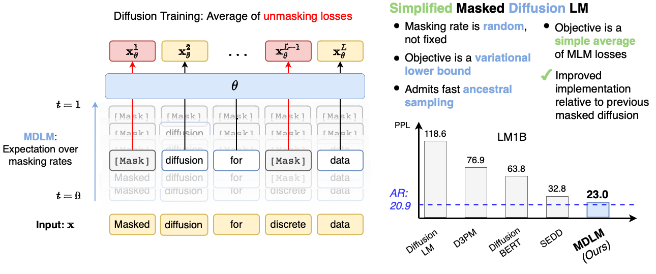
As shown in Figure 1, training can be read as “BERT with the mask rate treated as a random variable.”
Why Read MDLM First
The discrete diffusion framework presented by D3PM unifies a variety of transition matrices such as uniform / absorbing / discretized Gaussian, yet its objective function is written as a sum of Kullback-Leibler (KL) divergences, which does not make for the clearest implementation perspective. SEDD (Score Entropy Discrete Diffusion) (Lou et al. 2024) later reconstructed the objective from the viewpoint of concrete score / ratio matching, but the discrete-domain complications inherent in explicitly handling score functions remained.
Against this backdrop, MDLM showed that if one restricts to the absorbing transition (a one-way transition into the [MASK] state) and takes the continuous-time limit, then the evidence lower bound (ELBO) reduces to a masked cross-entropy weighted by \(1/t\). As a result,
- training can be implemented as a continuous-time generalization of BERT’s random mask prediction
- inference can be written as a sampling loop over discrete time steps
- the formulation structurally corresponds to denoising score matching in continuous diffusion models (Denoising Diffusion Probabilistic Models (DDPM), etc.)
This yields a remarkably clear picture. For grasping in one paper “what DLLM training actually is doing,” there is no better entry point than MDLM.
In the same year as MDLM, Shi et al. independently proposed a similar masked diffusion formulation (Shi et al. 2024). Although the notation differs, both arrive at essentially the same structure of “absorbing + continuous-time ELBO → weighted masked CE,” and today the two papers are often cited together.
Core of the Formulation
Notation
Let \(V\) denote the vocabulary size and \(L\) the sequence length, and write a clean sequence as \(x_0 = (x_0^1, \dots, x_0^L)\). Each token can take \(V+1\) states (the \(V\) regular vocabulary tokens plus the special token [MASK]). \(x_t^i\) denotes the token at position \(i\) at time \(t \in [0,1]\).
Forward Process
Each token position is independently replaced with [MASK] with probability \(t\). At \(t = 0\), \(x_0\) remains intact; at \(t = 1\), every position becomes [MASK]. For each position \(i\),
\[ q(x_t^i \mid x_0^i) = \begin{cases} 1 - t & x_t^i = x_0^i \\ t & x_t^i = \texttt{[MASK]} \end{cases} \]
This corresponds to the continuous-time version of the absorbing transition of D3PM in discrete time. Once a position becomes [MASK], it never reverts to the original token during the forward process (the absorbing property).
Reverse Process
The reverse process can be written as a one-step transition from \(t\) to \(t - \mathrm{d}t\) that fills in some of the [MASK] positions with predicted tokens. When position \(i\) is [MASK] at time \(t\), the conditional distribution at time \(s < t\) is
\[ q(x_s^i \mid x_t^i = \texttt{[MASK]}, x_0^i) = \begin{cases} \frac{t - s}{t} & x_s^i = x_0^i \\ \frac{s}{t} & x_s^i = \texttt{[MASK]} \end{cases} \]
In implementation, this true posterior is approximated by predicting \(x_0\) with a neural network \(p_\theta(x_0 \mid x_t)\). That is, the reverse process is learned in the spirit of \(x_0\)-prediction.
Objective Function
Instantiating the continuous-time ELBO integral under the forward / reverse process choices above, the loss ultimately reduces to the following.
Theorem 1 (The MDLM Objective (Sahoo et al. 2024)) Under the continuous-time absorbing forward process, the negative ELBO of MDLM is equivalent to the following loss.
\[ \mathcal{L}_\text{MDLM} = \mathbb{E}_{t \sim \mathcal{U}(0,1)} \, \mathbb{E}_{x_t \sim q(\cdot \mid x_0)} \left[ \frac{1}{t} \sum_{i=1}^{L} \mathbf{1}[x_t^i = \texttt{[MASK]}] \, \log p_\theta(x_0^i \mid x_t) \right] \tag{1}\]
The essential points here are the following two.
- Evaluated only at
[MASK]positions: due to \(\mathbf{1}[x_t^i = \texttt{[MASK]}]\), unmasked positions do not contribute to the loss - Weight \(1/t\): the smaller \(t\) (the fewer masks), the larger the contribution per mask
Theorem 1 is an extension of BERT’s random mask prediction loss in which “the mask rate is varied over \(t \in [0,1]\) and weighted by \(1/t\).” This is precisely why MDLM is said to be “a continuous-time version of BERT.”
Outline of Deriving the Training Objective
The detailed calculations are deferred to §3 and Appendix A of the original paper, but the logical skeleton leading to (Equation 1) is as follows.
Discrete-Time Version of the ELBO
Discretizing time as \(0 = t_0 < t_1 < \dots < t_N = 1\), the ELBO can be written as
\[ \log p_\theta(x_0) \geq -\mathbb{E}_q \left[ \sum_{n=1}^{N} D_\text{KL}\left( q(x_{t_{n-1}} \mid x_{t_n}, x_0) \,\big\|\, p_\theta(x_{t_{n-1}} \mid x_{t_n}) \right) \right] + \text{const.} \]
Each KL decomposes per position (because the forward process is position-independent).
Evaluating the KL at Each Position
The KL at position \(i\) splits into cases depending on whether \(x_{t_n}^i\) is [MASK] or a regular token.
- \(x_{t_n}^i \ne \texttt{[MASK]}\) (already determined): by the absorbing property, \(x_{t_{n-1}}^i = x_{t_n}^i\) is determined deterministically, so both the posterior and the prior become deltas and the KL is 0
- \(x_{t_n}^i = \texttt{[MASK]}\): the posterior is “fill with \(x_0^i\) with probability \((t_n - t_{n-1})/t_n\), remain
[MASK]with probability \(t_{n-1}/t_n\),” and only here does a non-trivial KL arise
The fact that the loss at unmasked positions vanishes stems precisely from the absorbing property. Information that has once “erupted” via the forward process into [MASK] is, if it remains [MASK] at time \(t\), undetermined (incurs loss); if it has disappeared, already determined (no loss). The structure is that simple.
Continuous-Time Limit
Taking the limit \(N \to \infty\), the step width \(\Delta t = t_n - t_{n-1}\) tends to 0, and the leading term of the KL is rearranged into the form
\[ \frac{\Delta t}{t_n} \cdot (- \log p_\theta(x_0^i \mid x_{t_n})). \]
Integrating this produces a \(1/t\) weighting in time \(t\). It is easier to build intuition if you think of the weight \(1/t\) as coming from the rate at which tokens are absorbed into [MASK] per unit time by the forward process, rather than from absolute time.
Denoising Loop at Inference Time
After training, sampling is performed by tracing the reverse process at discrete time steps. The basic form can be expressed by the following pseudocode.
# x_T: initialized with [MASK] at every position (T is the number of steps)
x = [MASK] * L
for t in linspace(1.0, 0.0, T+1)[:-1]:
    s = t - 1.0 / T
    # Prediction by the neural network p_theta
    logits = model(x)
    # Sample predictions only at MASK positions
    for i in masked_positions(x):
        if rand() < (t - s) / t:
            x[i] = sample(softmax(logits[i]))
        # else: leave as MASK
In this basic form, “each [MASK] position is fixed independently with probability \((t - s)/t\)”: increasing the step count \(T\) reduces the number fixed per step, raising quality. Conversely, reducing \(T\) is faster but degrades quality. \(T\) is the hyperparameter that governs the compute–quality trade-off.
In practice, rather than “fixing positions randomly with some probability,” a strategy of “fixing positions in order of highest prediction-logit confidence” is commonly used. This originates from MaskGIT in image generation and is adopted by subsequent models such as LLaDA. The theoretical reverse process of MDLM uses random fixing, but the choice of sampler can be swapped out independently of the theory.
→ Details: LLaDA: Large-Scale Masked DLM and Sampling
Why the Absorbing Transition Is the Natural Choice
D3PM could handle multiple transitions such as uniform / absorbing / discretized Gaussian, but MDLM deliberately restricts to absorbing. Why is this a natural choice?
The One-Way Property: “Erupted Information Does Not Return”
The essence of the absorbing process is that information loss is one-way. Once a position becomes [MASK], it does not revert to another token or change into a different regular token during the forward process. This makes possible the following:
- in the reverse process, one can make a simple distinction: “positions currently
[MASK]have an unknown original value” vs “positions with a regular token retain the original” - the learning objective only needs to be evaluated at
[MASK]positions - it corresponds directly to BERT’s mask prediction task
In the uniform transition case (replacement with an arbitrary token), the reverse process needs to distinguish “currently token \(a\), but is that the original \(a\) or did some other character change into it?,” which complicates the objective function. Absorbing is the choice that simultaneously yields a “simple objective function” and a “connection to BERT.”
Compatibility with Language Data
In language data, “a particular token is replaced with [MASK]” corresponds naturally to operations like missing values, redactions, or fill-in-the-blank. It fits text-processing intuition better than uniform replacement (substituting some other random token).
Experimental Results and Scaling
The MDLM paper shows the following points through experiments on LM1B and OpenWebText.
| Comparison target | Position of MDLM |
|---|---|
| D3PM (absorbing) | Achieves better perplexity |
| SEDD | On par or better, with a simpler implementation |
| AR (GPT-2 of comparable scale) | Slightly worse, but scales comparably |
Especially important is that performance improves following scaling laws similar to AR. That is, the decrease in perplexity as compute, data, and model size increase exhibits a pattern similar to AR, suggesting that DLLMs are not “toys that only work at small scale.” This observation also motivates the later LLaDA work (at the 8B scale).
Reading Priority
The table below summarizes the importance of each section when reading the paper.
| Section | Importance | Content |
|---|---|---|
| §2 Formulation | Must read (multiple passes) | Definitions of forward / reverse processes, notation |
| §3.1 Derivation of the objective | Must read | Simplification from the ELBO to the \(1/t\)-weighted CE |
| §3.2 SUBS parameterization | Recommended | Design of the \(x_0\)-prediction head, trick to zero out [MASK] output |
| §4 Sampling | Must read | Inference loop, ancestral / analytic samplers |
| §5 Experiments | Skim is enough | LM1B / OWT / zero-shot perplexity |
| Appendix A | Scan is enough | Proof of D3PM equivalence, rigorous treatment of the continuous-time limit |
| Appendix B–C | Reference | Derived losses, implementation details |
In particular, §2 and §3.1 are prerequisites for reading the other chapters in this book, so aim to read them at least twice and reach a state where you can explain in your own words “the definition of the forward process” and “why the ELBO becomes a CE evaluated only at [MASK] positions.”
What You Will Understand After Reading This Paper
A first pass through MDLM yields the following understanding.
- The true nature of DLLM training: it is fair to think of it simply as “BERT training with a noise schedule.” Apart from sampling the mask rate \(t\) uniformly and weighting by \(1/t\), there is essentially no difference from BERT.
- The meaning of denoising steps at inference: it is sampling at discrete time steps \(t_n\), and the step count \(T\) is a hyperparameter that trades off compute against quality. In theory, \(T \to \infty\) approaches the continuous-time reverse process.
- The role of the absorbing property: the property that “once unmasked, it is fixed” is the fundamental reason the objective simplifies to evaluation only at
[MASK]positions. - Relation to AR: AR can be viewed as one-directional unmasking from left to right (predicting tokens sequentially), and DLLMs can be viewed as a generalization to order-free unmasking.
Correspondence with Continuous Diffusion Models
Denoising score matching (DSM) in continuous diffusion (DDPM, VP-SDE, etc.) takes the form of an L2 loss weighted by the noise strength \(\sigma_t\),
\[ \mathcal{L}_\text{DSM} = \mathbb{E}_t \, \mathbb{E}_{x_t} \left[ w(t) \, \| s_\theta(x_t, t) - \nabla_{x_t} \log q(x_t \mid x_0) \|^2 \right] \]
The MDLM objective (Equation 1) is structurally isomorphic to this.
| Continuous diffusion (DSM) | MDLM |
|---|---|
| L2 loss (regression of the score \(s_\theta\)) | Masked cross-entropy (\(x_0\)-prediction) |
| Noise-dependent weight \(w(t)\) | Time-dependent weight \(1/t\) |
| Forward: add Gaussian noise | Forward: mask with probability \(t\) |
| Reverse: SDE / ODE integration | Reverse: discrete-time unmasking |
Both share the spirit of “learning the reverse process via \(x_0\)-prediction,” and the difference in the weight structure of the loss appears as the contrast between “weighted regression vs weighted classification.” Viewing them this way provides a unified perspective.
→ Details: Continuous vs Discrete Diffusion: Bridging the Two