LDT

The Lattice Deduction Transformer (LDT) is a recursive reasoning model proposed in a May 2026 paper by Liam Davis at Amherst College, Leopold Haller and Alberto Alfarano at Axiom, and Mark Santolucito at Barnard College / Columbia University (Davis et al. 2026). The point can be stated in one line. By projecting the latent state of a recurrent transformer onto the lattice of abstract interpretation after every forward pass, LDT obtains sound deduction (returning the correct answer or otherwise abstaining) rather than approximate refinement. An 800K-parameter LDT solves Sudoku-Extreme and Snowflake Sudoku at 100 % / 100 %, and a 1.8M-parameter variant solves Maze-Hard at 99.9 %, while Frontier Large Language Models (LLMs) such as Claude Opus 4.6, DeepSeek V4-Pro 1.6T, and GPT-5.4 all score 0 %. Against the “approximate refinement” lineage of HRM, TRM, PTRM, and GRAM covered in this book, LDT stakes out an independent position as the “sound deduction” lineage. Genealogically it sits at the end of HRM to TRM to Sotaku to LDT, and can be read as inheriting Sotaku’s architecture and adding lattice projection on top to turn approximation into soundness.

Lineage: Independent Evolution via Sotaku

The direct predecessor of LDT is Sotaku, implemented by Cheng Lou as an individual project (2026, (Lou 2026)). Sotaku is a roughly 800K-parameter neural network (NN) that combines a 4-layer weight-shared transformer with 2D Rotary Position Embedding (RoPE) (Su et al. 2024), and it achieves 98.9 % (24728/25000) on Sudoku-Extreme under a test-time scaling setup of 16 internal iterations at training and 1024 at inference. Its important feature is that it is Sudoku-agnostic: it does not use row / col / box constraint embeddings and assumes only a pure 2D grid. Compared with Samsung TinyRecursiveModels’ TRM, which achieves 87.4 % at 7M parameters, Sotaku independently reaches 11 points higher accuracy at one tenth the size.

LDT inherits this Sotaku base architecture (looped transformer plus 2D RoPE) almost as-is. On top of that inheritance, it adds the lattice projection of abstract interpretation to turn Sotaku’s approximation into soundness. Read as a branching point off the TRM lineage covered in the TRM chapter, Sotaku sits at the “extreme of size reduction and simplification” and LDT at the “extension that adds soundness guarantees on top”.

flowchart TB
    HRM["HRM (27M)<br/>approximate refinement"] --> TRM["TRM (7M)<br/>approximate refinement"]
    TRM --> Sotaku["Sotaku (800K)<br/>approximate refinement"]
    TRM --> PTRM["PTRM<br/>approximate +<br/>test-time noise"]
    TRM --> GRAM["GRAM<br/>approximate +<br/>generative"]
    Sotaku --> LDT["<b>LDT (800K)</b><br/><b>sound deduction</b>"]

Figure 1: The lineage and classification of the five papers covered in this book. HRM, TRM, PTRM, and GRAM are the approximate refinement lineage, treating the latent state as an opaque hidden state. Sotaku is the minimization endpoint of the TRM lineage, and LDT branches off into the sound deduction lineage by inheriting Sotaku’s architecture and adding lattice projection.

The Lattice of Abstract Interpretation

Abstract interpretation is the framework Cousot and Cousot introduced in 1977 for program analysis (Cousot and Cousot 1977), a general theory for soundly over-approximating properties on an expensive concrete domain \(C\) over a more tractable abstract domain \(A\). We organize just the minimal vocabulary that LDT needs.

The two domains are connected by a Galois connection \((\alpha, \gamma)\). \(\alpha : C \to A\) is abstraction (how information is dropped) and \(\gamma : A \to C\) is concretization (the set of concrete points that an abstract point represents), satisfying \(S \subseteq \gamma(\alpha(S))\) and \(\alpha(\gamma(a)) \sqsubseteq a\). The order \(\sqsubseteq\) is read as precision, \(\top\) is the state of knowing nothing (all candidates still alive), and \(\bot\) corresponds to the inconsistent state (no solution). Deduction is the monotone task of descending from \(\top\) and narrowing information, and collapsing to \(\bot\) is conflict detection. Being sound means “any claim derived on the abstract holds on the concrete as well”, at the cost of losing completeness (some properties that are true on the concrete cannot be derived on the abstract).

LDT’s concrete instantiation for Sudoku is as follows. The concrete domain is the powerset of the set of complete solutions \(G = \{1,\dots,9\}^{81}\), and the abstract domain is the grid powerset lattice

\[ A = (\{1,\dots,9\}^2 \to 2^{\{1,\dots,9\}}) \]

that is, each cell carries a “set of candidates still alive”. A solution is one-hot, \(\alpha\) is the bit-level OR over a set, and \(\gamma\) is “the set of all complete solutions consistent with the candidate set at each cell”. As Appendix A of the paper shows, the grid powerset lattice discards inter-cell correlations, so \(\gamma(\alpha(S))\) is typically a larger set than the original \(S\). Even so, running deduction (monotone removal of candidates) on this abstract leaves only sound information.

The most precise sound deduction is

\[ \mathrm{ded}_p(a) = \alpha\bigl(\gamma(a) \cap \|p\|\bigr) \]

where \(\|p\|\) is the solution set of puzzle \(p\). LDT approximates this \(\mathrm{ded}_p\) with a transformer. Naked single and hidden single are examples of weak hand-built sound abstract deductions, and LDT’s goal is to learn \(\mathrm{ded}_p\) itself.

flowchart LR
    C["<b>Concrete domain C</b><br/>set of complete solutions<br/>powerset of grids"] -- "α (abstraction)" --> A["<b>Abstract domain A</b><br/>grid powerset lattice<br/>per-cell candidate sets"]
    A -- "γ (concretization)" --> C
    A -.-> Top["⊤: all candidates alive"]
    A -.-> Bot["⊥: conflict"]

Figure 2: Conceptual diagram of the Galois connection \((\alpha, \gamma)\). Between the concrete domain C and the abstract domain A, abstraction \(\alpha\) and concretization \(\gamma\) form an adjoint pair. For Sudoku, C is the set of complete solutions, A is the per-cell candidate-set lattice, \(\top\) represents all candidates alive, and \(\bot\) represents a conflict.

NoteLateral Move from Program Analysis to Logical Deduction

Abstract interpretation was originally developed as a theory of program analysis, where its native use is to compute fixed points of monotone transformers over program states on the abstract domain. What LDT shows is the observation that the same theory applies naturally to logical deduction. There is a difference in convention, in that program analysis takes the least fixed point while LDT takes the greatest, but as the authors themselves note at the end of the paper’s Appendix A, “abstract interpretation is a theory of sound approximation for inferential computation in general, and the program-semantics framing is just one of its applications”. The Sudoku setting covered in this chapter is another such application, on the side of logical deduction, constraint satisfaction, and puzzle solving.

Architecture

Lattice Encoding

LDT encodes the grid powerset lattice as a tensor input to the transformer (paper Section 4.1). For a 9x9 Sudoku, it carries \(9 \times 9 \times 9 = 729\) binary sigmoids, each representing “the confidence that this candidate is still alive at this cell”. A solution is one-hot (only one digit alive per cell), and \(\alpha\) is the bit-level OR per cell. In addition, a single CLS sigmoid is placed as a “conflict detection head”. Once it exceeds a threshold \(\theta_{\mathrm{CLS}}\), the current lattice state is judged as “non-concretizable (\(\bot\))” and triggers backtracking.

For the variable-topology problem Snowflake Sudoku, the model prepares a fixed \(15 \times 10\) covering grid and adds a read-only in-puzzle mask channel per cell. This lets it handle different hexagonal topologies from \(n=3\) to \(n=7\) (18 to 90 cells) with the same model and no architectural changes.

Recurrent Transformer (Sotaku Style)

The NN part follows Sotaku almost as-is. A 4-layer attention block is unrolled across 16 internal iterations, with each iteration’s output feeding the next iteration’s input. The input lattice encoding is re-injected as a residual at every iteration. Position information is supplied as a learned 2D positional embedding added to the input, and for the \(30 \times 30\) Maze grid, 2D RoPE (Su et al. 2024) is added inside attention. Each iteration outputs candidate logits and a CLS logit independently. At training, loss is applied to all 16 iterations (deep supervision), and at inference only the final iteration is read.

NoteContrast with TRM / HRM / Sotaku

HRM has four components (input network, low-level recurrent module, high-level recurrent module, output head) and a dual recursion. TRM unrolls a single 2-layer network deeply with weight tying. Sotaku trims the TRM lineage further, collapsing it into 4-layer weight-shared blocks plus 2D RoPE. LDT inherits this Sotaku architecture almost entirely and adds soundness by inserting lattice projection between forward passes. That is, it is not the expressive power of the NN but the act of projecting the NN’s output state onto the lattice at every step that guarantees soundness.

Solve Loop: Unified Procedure for Training and Inference

The central design of LDT is the Solve loop in Section 4.2. The same procedure advances the lattice state at both training and inference. One step is summarized by the pseudocode below.

# Algorithm 1: Solve (used for both training and inference)
def solve(x_0, Y):  # Y: ground-truth solutions, empty at inference
    x = x_0
    while True:
        x_new, conflict, solved, loss = step(x, Y)
        if Y:  # training only
            optimizer_step(loss)
        x = x_new
        if conflict or solved:
            return x, conflict, solved

# Algorithm 2: step operator
def step(x, Y):
    # (i) 4-layer transformer x 16 internal iterations on lattice state x
    b, c = transformer_forward(x)
    # (ii) eliminate candidates with confidence below theta_elim
    x_new = eliminate(x, sigmoid(b) < theta_elim)
    conflict = (sigmoid(c) > theta_CLS) or has_empty_cell(x_new)
    solved   = all_cells_singleton(x_new) and not conflict
    if Y:
        target = x_new & alpha({y for y in Y if consistent(y, x_new)})
        loss   = bce_asym(b, target) + lambda_cls * bce(c, conflict) + lambda_ce * ce(b, target)
    # (iii) if neither conflict nor solved, randomly pick a multi-candidate cell
    # and pin one digit sampled from softmax of its candidate confidences
    if not conflict and not solved:
        x_new = sample_branch(x_new, tau_decide)
    return x_new, conflict, solved, loss

The step operator consists of three stages: (i) a transformer forward pass with 16 internal iterations producing candidate and CLS logits, (ii) elimination of candidates whose confidence falls below \(\theta_{\mathrm{elim}}\), and (iii) if neither terminal condition holds, uniformly sampling a cell with multiple remaining candidates and pinning one digit drawn from the softmax of its candidate confidences. Termination is either conflict or solved, and termination is guaranteed because the lattice set is finite and each step must reduce the candidate count.

Using the same procedure at training and inference is the central design decision of the Solve loop. It is a device to align “the distribution of lattice states the model sees at training” with “the distribution of states it encounters at inference”, and the paper positions it as “halfway between on-policy distillation (Agarwal et al. 2024) and standard supervised fine-tuning”. The teacher signal is supplied state-conditionally by the alpha operator hitting the set of ground-truth solutions consistent with the current state \(x\). Unlike HRM / TRM / PTRM / GRAM, which carry a latent embedding across segments, LDT lets the lattice itself carry the state, so gradients do not flow between steps. Combining cross-step latents is explicitly listed as future work.

Loss Design

The deep supervision at each iteration combines three losses.

\[ \mathcal{L} = \frac{1}{L} \sum_{\ell=1}^{L} \Bigl[ \mathcal{L}_{\mathrm{BCE}}^{(\ell)} + \lambda_{\mathrm{cls}} \mathcal{L}_{\mathrm{CLS}}^{(\ell)} + \lambda_{\mathrm{ce}} \mathcal{L}_{\mathrm{CE}}^{(\ell)} \Bigr] \]

The first term is an asymmetric Binary Cross Entropy (BCE) on the candidate sigmoids, with positive-class weight \(w^+\) and negative-class weight \(w^-\) set so that \(w^+ / w^- = 8\). This means “wrongly killing a correct candidate” is penalized 8 times more heavily than “leaving a false candidate alive”, directly embodying the engineering choice to prioritize soundness over completeness. The paper adopts \(w^+ / w^- = 8, \lambda_{\mathrm{cls}} = 0.1, \lambda_{\mathrm{ce}} = 0.2, \theta_{\mathrm{elim}} \approx 0.1, \tau_{\mathrm{decide}} = 1.5\) for Sudoku and transfers them to other domains without modification. The second term is a symmetric BCE between the CLS sigmoid and the indicator of “whether the current state has collapsed to \(\bot\)”, and the third is a softmax CE applied to cells that have become singletons, introduced only to accelerate convergence.

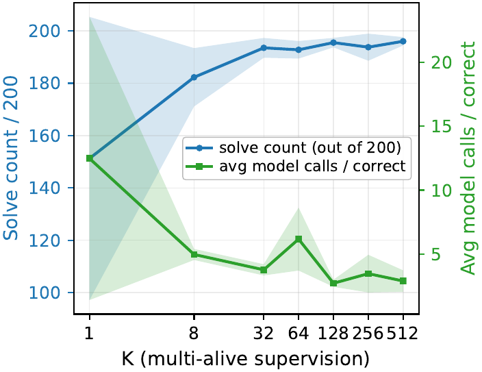
Handling Multiple Solutions: The Alpha Operator

When the same puzzle admits multiple shortest paths, as in Maze, fixing a single ground truth penalizes equivalent correct solutions. LDT handles this naturally through the alpha operator. It pre-samples \(K\) valid solutions per puzzle and supervises with the supervision target obtained by applying \(\alpha\) to the subset consistent with the current state \(x\):

\[ \hat{y} = x \sqcap \alpha\bigl(\{y \in Y \mid y \text{ is consistent with } x\}\bigr) \]

For \(K=1\) this reduces to ordinary single-target supervised learning. While the remaining consistent solution set is still multiple for \(K > 1\), \(\hat y\) stays multi-alive, and it collapses to one-hot once the state commits to the path of a single solution. In abstract interpretation terms, this corresponds to taking the “join” of the solution set on the abstract domain.

Main Results

Sudoku-Extreme: 100% Soundness with 800K Parameters

Sudoku-Extreme in paper Table 1 is the same benchmark as in the HRM paper, a collection of hard puzzles requiring an average of 22 backtracks. Training an 800K-parameter LDT on the 1K-puzzle train split for 4K steps (15 minutes on a single B200 GPU) brings both soundness and accuracy to 100 / 100. The comparison points are as follows.

Table 1: Comparison on Sudoku-Extreme. The three Frontier LLMs cannot solve a single puzzle. LDT reaches 100 % soundness at 1/10 to 1/30 the size of TRM / HRM and with 1/2700 the training data of Sotaku, and even without augmentation accuracy stays at 99.7 % while soundness remains 100 %.

Method	Parameters	Train	Soundness / Accuracy (%)	Train cost
Claude Opus 4.6	?	-	0.0 / 0.0	-
DeepSeek V4-Pro	1.6T	-	0.0 / 0.0	-
GPT-5.4	?	-	0.0 / 0.0	-
HRM	27M	1K	55.0 / 55.0	-
TRM	5M	1K	87.4 / 87.4	36h (4x L40S)
Sotaku	800K	2.7M	98.9 / 98.9	2h40m (1x H100)
LDT, 4K steps	800K	1K	100 / 100	15min (1x B200)
LDT, 4K steps (no-aug)	800K	1K (no-aug)	100 / 99.7	13min (1x B200)

Four points are worth noting. First, the fact that all three Frontier LLMs score 0 / 0 reaffirms that “problems solvable by scale” and “problems solvable by small recurrent reasoners” do not overlap (the same observation as in the HRM / TRM chapters). Second, LDT undercuts the parameter count of TRM / HRM by orders of magnitude. Third, while Sotaku required 2.7M puzzles for training, LDT uses only 1K puzzles at the same 800K size. Fourth, even with puzzle augmentation removed entirely, accuracy stays at 99.7 % and soundness stays at 100 %. TRM diverged on Sudoku unless 1000 augmentations were applied, but in LDT the soundness of abstract interpretation takes over the role that augmentation played.

Figure 3: Train-compute vs. test-compute tradeoff on Sudoku-Extreme. As training steps increase, the median and upper percentiles of per-puzzle forward passes at inference shrink by orders of magnitude. Soundness stays at roughly 100 %, while only the test compute drops. Source: (Davis et al. 2026)

Figure 4: Distribution of per-puzzle forward passes on Sudoku-Extreme. It is bimodal, with the left peak corresponding to a “deduction mode” solvable by lattice projection alone and the right peak to a “search mode” that requires branching. More training shifts mass to the deduction mode (left). Source: (Davis et al. 2026)

Snowflake Sudoku: Generalization to Variable Topologies

Section 5.2 of the paper tests generalization to Snowflake Sudoku, a hexagonal Sudoku variant. Puzzles with different topologies from \(n=3\) to \(n=7\) (18 to 90 cells) are synthesized as 30,000 instances using the cvc5 SMT solver (Barbosa et al. 2022), with 500 used for training and 1000 for test (LLMs are evaluated only on 200 puzzles for compute reasons). An 800K LDT trained on 500 puzzles reaches 100 / 100, while Claude Opus 4.6 / DeepSeek V4-Pro / GPT-5.4 again all fail. What is notable as generalization of sound deduction to variable topologies is that a single model handles every size from \(n=4\) to \(n=7\) using only the \(15 \times 10\) covering grid and a per-cell mask channel.

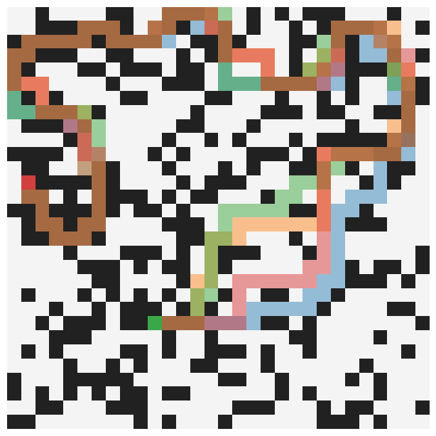
Maze-Hard: Application to Multi-Solution Tasks

Section 5.3 of the paper tests multi-solution supervision on \(30 \times 30\) Maze-Hard (shortest path length \(\geq 110\)). LDT 1.8M (embedding dimension \(d = 192\)) reaches 99.3 / 99.3 at \(K=1\) and 99.9 / 99.9 at \(K=512\), while HRM stays at 74.5 and TRM at 85.3. One caveat is that on Maze, LDT is not fully sound either. In 1 / 1000 failures it does not abstain but returns a “correct but not shortest” path. That is not an error in the sense that it is still a valid path, but it is an error under the benchmark’s “shortest path” criterion, and the paper itself states this candidly as a limitation.

Figure 5: Example of Maze-Hard (\(30 \times 30\)). The start, the goal, and multiple shortest paths of equal length coexist. LDT samples \(K\) valid solutions via the alpha operator and uses their common part as the supervision target, handling multiple solutions naturally. Source: (Davis et al. 2026)

Figure 6: The \(K\) sweep for multi-solution supervision on Maze-Hard. As \(K\) grows, the solve rate (blue, left axis) rises and the mean number of forward passes per puzzle (green, right axis) shrinks. Most of the gain is recovered at small \(K\), and it saturates around \(K \geq 32\). Source: (Davis et al. 2026)

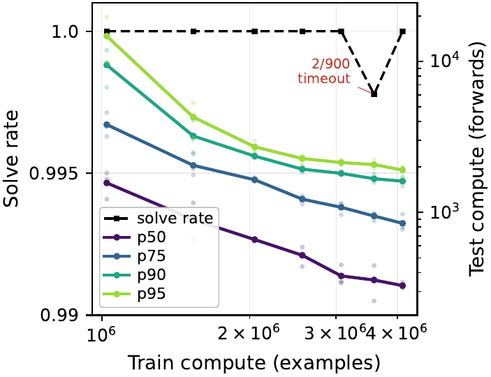
Implications of the Train / Test Compute Tradeoff

Figure 3 contains a result that deserves to be reread in the broader context of this book. The claim that “as training compute grows, both the median and upper percentiles of inference-time forward passes shrink by orders of magnitude” runs in the opposite direction from sequential token scaling by CoT and from the recurrent depth scaling shown by HRM / TRM / GRAM. Frontier LLMs like OpenAI o1 / DeepSeek-R1 (DeepSeek-AI et al. 2025) try to solve hard problems by “thinking longer (= generating more tokens)”, and HRM / TRM try to gain effective depth by increasing recursion depth at test time. What LDT shows is a new tradeoff: once sound deduction can be learned, additional training works in the direction of taking over and removing inference-time search.

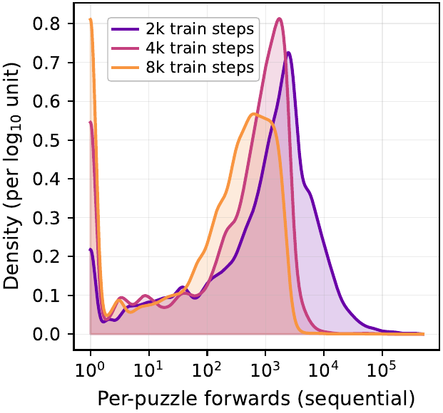
Why is that possible. Lattice projection guarantees soundness, which lets the model concentrate on “learning accurate deduction”. In contrast, the approximate refinement lineage has no guarantee that the answer is correct even when training proceeds well, and must compensate with test-time search or denoising steps. As the bimodal distribution in Figure 4 shows, more training shifts mass toward the “deduction mode” solvable by lattice projection alone, and the “search mode” peak that requires branching itself moves toward shorter forward counts. This observation adds a new axis to the test-time compute allocation discussion covered in Depth vs Token Scaling: with sound deduction, search can be internalized through training.

Related Work

Haller’s Prior Work: Author Continuity

Co-author Leopold Haller of LDT is the same Haller of D’Silva, Haller, and Kroening’s 2013 POPL paper on Abstract Conflict Driven Learning (ACDL) (D’Silva et al. 2013). ACDL lifts Conflict-Driven Clause Learning (CDCL) (Marques-Silva et al. 2009), the standard technique of modern SAT solvers, to a lattice-theoretic formulation as a decision problem for distributive transformers over Boolean lattices. It is a reconstruction in the vocabulary of abstract interpretation of the operating principle of CDCL, where a “learned clause that excludes the failure” is generated on every conflict.

Viewed from here, LDT’s CLS conflict head can be read as effectively a learned version of ACDL. It is an attempt to have a neural network learn an equivalent role to the mechanism by which a Boolean Satisfiability (SAT) solver detects conflicts and cuts back branches. The paper does not explicitly write “LDT is the neuralization of ACDL”, but from both the author continuity and the architectural correspondence, this is the natural medium- to long-term lineage in which to read it.

Neuro-Symbolic Logical Reasoning

There are two research lineages close to LDT. The first embeds an exact solver as a network layer. SATNet (P.-W. Wang et al. 2019) embeds a differentiable relaxation of a MAX-SAT solver, and Learning Modulo Theories (Fredrikson et al. 2023) embeds a Satisfiability Modulo Theories (SMT) solver, each as a layer of an NN. The difference from LDT is that SATNet / LMT place a differentiable solver inside the NN, while LDT guarantees soundness only through the non-differentiable structural constraint of lattice projection and lets the NN learn freely. As design philosophies they are contrasts.

The second is the “abstract interpretation x ML” lineage centered around the Singh lab. Neural Abstract Interpretation (NAI) (Gomber and Singh 2025) is the closest immediate precursor in spirit, proposing a frame for learning a neural net as an abstract transformer. The difference is the level of integration: NAI trains the transformer alone for program analysis, while LDT integrates the entire iterative deduction with a looped transformer plus lattice projection. LAIT (He et al. 2020) and SAIL (Gu et al. 2026) are in the same lineage, with SAIL using an LLM to learn abstract interpreters.

Affinity with Diffusion

Sections 1 and 2 of the paper emphasize the structural affinity between lattice projection and discrete diffusion. D3PM (Austin et al. 2021) learns a forward process with a transition matrix into an absorbing state and iteratively commits partial information in the reverse process. LDT’s lattice projection is the operation of “shrinking the current candidate set” and can be read as a D3PM whose transition matrix is restricted to lattice-respecting ones. ReMDM (G. Wang et al. 2025) is a discrete diffusion that lets generated tokens be re-masked at inference time, which corresponds to branching and backtracking in LDT. The paper does not develop LDT as diffusion methodology, but leaves the observation “lattice projection is isomorphic to denoising” as a foothold for future work.

As contemporaneous work, Constraints-Guided Diffusion Reasoner (CGDR) (Zhang et al. 2025) realizes neuro-symbolic learning on the same Sudoku / Maze with discrete diffusion plus reinforcement learning via proximal policy optimization (PPO). Where LDT guarantees soundness with abstract interpretation, CGDR acquires constraint compliance with diffusion plus PPO, and the two can be contrasted as different approaches to the same goal.

Independence from the HRM / TRM / PTRM / GRAM Lineage

The fundamental difference between the previous four chapters of this book and LDT lies in the interpretation and guarantees of the latent state. HRM / TRM / PTRM / GRAM treat the latent state as an opaque hidden state and run approximate refinement on top. They produce answers, but there is no guarantee that the answer is correct. LDT, in contrast, treats the latent state as an interpretable element of the lattice and runs sound deduction. It either produces an answer or abstains, never producing an incorrect one (empirically).

Both belong to the same “small recurrent transformer” architecture family, but their design philosophies are fundamentally different. The direction of PTRM, which adds test-time noise to TRM to escape bad basins, and the direction of LDT, which projects the latent onto a lattice to make it sound, should be read side by side as two orthogonal strategies for breaking through the limits of the TRM lineage. The former strengthens test-time exploration within the frame of approximate refinement, while the latter replaces the approximate nature itself with soundness.

Limitations

Section 6 of the paper lists three explicit limitations.

1. Restricted to tasks with explicit logical structure. In settings like the Abstraction and Reasoning Corpus (ARC)-AGI, where “rules are inferred for each task from a small number of demonstrations”, a naive port of LDT plateaus at roughly 36 % pass rate and the test-time search gain disappears as well. The reason is that the conflict head becomes unreliable and branching can no longer distinguish “good branches” from “bad branches”, and the paper describes ARC-AGI as “a representative setting in which LDT cannot be applied directly”.

2. Lattice design is task-dependent. The grid powerset lattice for Sudoku is hand-designed, and the extension to Snowflake was also done manually. Generalization to arbitrary tasks requires domain-specific abstract domain design, which is a general challenge of abstract interpretation as well.

3. No cross-step gradient flow. Gradients do not flow between steps of the Solve loop, and the lattice itself carries the state. Combining a TRM-style deep supervision across steps is untested and left as a future direction.

In settings like ARC, where rules are inferred from demonstrations, the paper suggests at the end that one may need to build the abstract domain not over “sets of solutions” but over “sets of programs that generate solutions”. Positioned in the context of this book, LDT can be read as the first paper that directly answers the engineering question that the HRM / TRM lineage implicitly avoided: “can we guarantee what kind of answer we returned”. More than the absolute performance number (100 % on Sudoku-Extreme), the contribution that is likely to matter most in the medium to long term is that it introduced soundness guarantees as a new evaluation axis into the discussion of recursive reasoning models.

References

Agarwal, Rishabh, Nino Vieillard, Yongchao Zhou, et al. 2024. “On-Policy Distillation of Language Models: Learning from Self-Generated Mistakes.” International Conference on Learning Representations (ICLR). https://arxiv.org/abs/2306.13649.

Austin, Jacob, Daniel D. Johnson, Jonathan Ho, Daniel Tarlow, and Rianne van den Berg. 2021. “Structured Denoising Diffusion Models in Discrete State-Spaces.” Advances in Neural Information Processing Systems (NeurIPS). https://arxiv.org/abs/2107.03006.

Barbosa, Haniel, Clark W. Barrett, Martin Brain, et al. 2022. “Cvc5: A Versatile and Industrial-Strength SMT Solver.” Tools and Algorithms for the Construction and Analysis of Systems (TACAS), Lecture notes in computer science, vol. 13243: 415–42. https://doi.org/10.1007/978-3-030-99524-9_24.

Cousot, Patrick, and Radhia Cousot. 1977. “Abstract Interpretation: A Unified Lattice Model for Static Analysis of Programs by Construction or Approximation of Fixpoints.” Conference Record of the Fourth Annual ACM SIGPLAN-SIGACT Symposium on Principles of Programming Languages (POPL) (Los Angeles, California), 238–52. https://doi.org/10.1145/512950.512973.

D’Silva, Vijay, Leopold Haller, and Daniel Kroening. 2013. “Abstract Conflict Driven Learning.” Proceedings of the 40th Annual ACM SIGPLAN-SIGACT Symposium on Principles of Programming Languages (POPL), 143–54. https://doi.org/10.1145/2429069.2429087.

Davis, Liam, Leopold Haller, Alberto Alfarano, and Mark Santolucito. 2026. “Lattice Deduction Transformers.” arXiv Preprint arXiv:2605.08605. https://arxiv.org/abs/2605.08605.

DeepSeek-AI, Daya Guo, Dejian Yang, et al. 2025. “DeepSeek-R1: Incentivizing Reasoning Capability in LLMs via Reinforcement Learning.” Nature 645: 633–38. https://arxiv.org/abs/2501.12948.

Fredrikson, Matt, Kaiji Lu, Saranya Vijayakumar, Somesh Jha, Vijay Ganesh, and Zifan Wang. 2023. “Learning Modulo Theories.” arXiv Preprint arXiv:2301.11435. https://arxiv.org/abs/2301.11435.

Gomber, Shaurya, and Gagandeep Singh. 2025. “Neural Abstract Interpretation.” ICLR 2025 Workshop: VerifAI: AI Verification in the Wild. https://openreview.net/forum?id=WTyyhWhp4m.

Gu, Qiuhan, Avaljot Singh, and Gagandeep Singh. 2026. “SAIL: Sound Abstract Interpreters with LLMs.” Proceedings of the ACM on Programming Languages 10 (PLDI).

He, Jingxuan, Gagandeep Singh, Markus Püschel, and Martin Vechev. 2020. “Learning Fast and Precise Numerical Analysis.” Proceedings of the 41st ACM SIGPLAN Conference on Programming Language Design and Implementation (PLDI), 1112–27. https://doi.org/10.1145/3385412.3386016.

Lou, Cheng. 2026. Sotaku: From-Scratch Experiments on Iterative Neural Sudoku Solvers. Software, GitHub repository, commit 9e13341. https://github.com/chenglou/sotaku.

Marques-Silva, João P., Inês Lynce, and Sharad Malik. 2009. “Conflict-Driven Clause Learning SAT Solvers.” In Handbook of Satisfiability, edited by Armin Biere, Marijn Heule, Hans van Maaren, and Toby Walsh, vol. 185. Frontiers in Artificial Intelligence and Applications. IOS Press. https://doi.org/10.3233/978-1-58603-929-5-131.

Su, Jianlin, Murtadha Ahmed, Yu Lu, Shengfeng Pan, Wen Bo, and Yunfeng Liu. 2024. “RoFormer: Enhanced Transformer with Rotary Position Embedding.” Neurocomputing 568: 127063. https://arxiv.org/abs/2104.09864.

Wang, Guanghan, Yair Schiff, Subham Sekhar Sahoo, and Volodymyr Kuleshov. 2025. “Remasking Discrete Diffusion Models with Inference-Time Scaling.” Advances in Neural Information Processing Systems (NeurIPS). https://arxiv.org/abs/2503.00307.

Wang, Po-Wei, Priya L. Donti, Bryan Wilder, and J. Zico Kolter. 2019. “SATNet: Bridging Deep Learning and Logical Reasoning Using a Differentiable Satisfiability Solver.” Proceedings of the 36th International Conference on Machine Learning (ICML), Proceedings of machine learning research, vol. 97: 6545–54. https://arxiv.org/abs/1905.12149.

Zhang, Xuan, Zhijian Zhou, Weidi Xu, Yanting Miao, Chao Qu, and Yuan Qi. 2025. “Constraints-Guided Diffusion Reasoner for Neuro-Symbolic Learning.” arXiv Preprint arXiv:2508.16524. https://arxiv.org/abs/2508.16524.